Đồ thị scatterplot

Từ khóa: đồ thị phân tán; plot xy; đồ thị điểm

Câu 1

Bạn có dữ liệu sau về chỉ số đo lường chất lượng không khí.

airquality -> df

head(df)
  Ozone Solar.R Wind Temp Month Day
1    41     190  7.4   67     5   1
2    36     118  8.0   72     5   2
3    12     149 12.6   74     5   3
4    18     313 11.5   62     5   4
5    NA      NA 14.3   56     5   5
6    28      NA 14.9   66     5   6

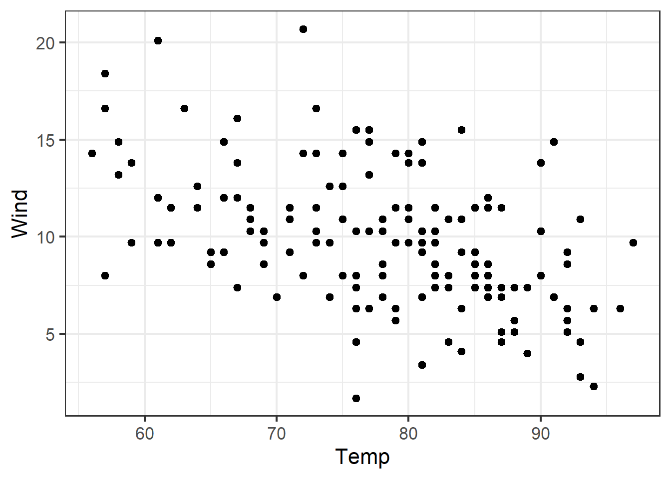
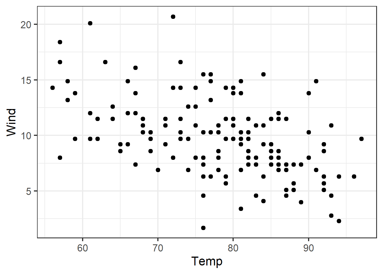
Bạn hãy vẽ đồ thị như hình bên dưới.

library(ggplot2)

ggplot(data = df,
       mapping = aes(x = Temp,
                     y = Wind)) +
  
  geom_point() +
  
  theme_bw(base_size = 16)

Câu 2

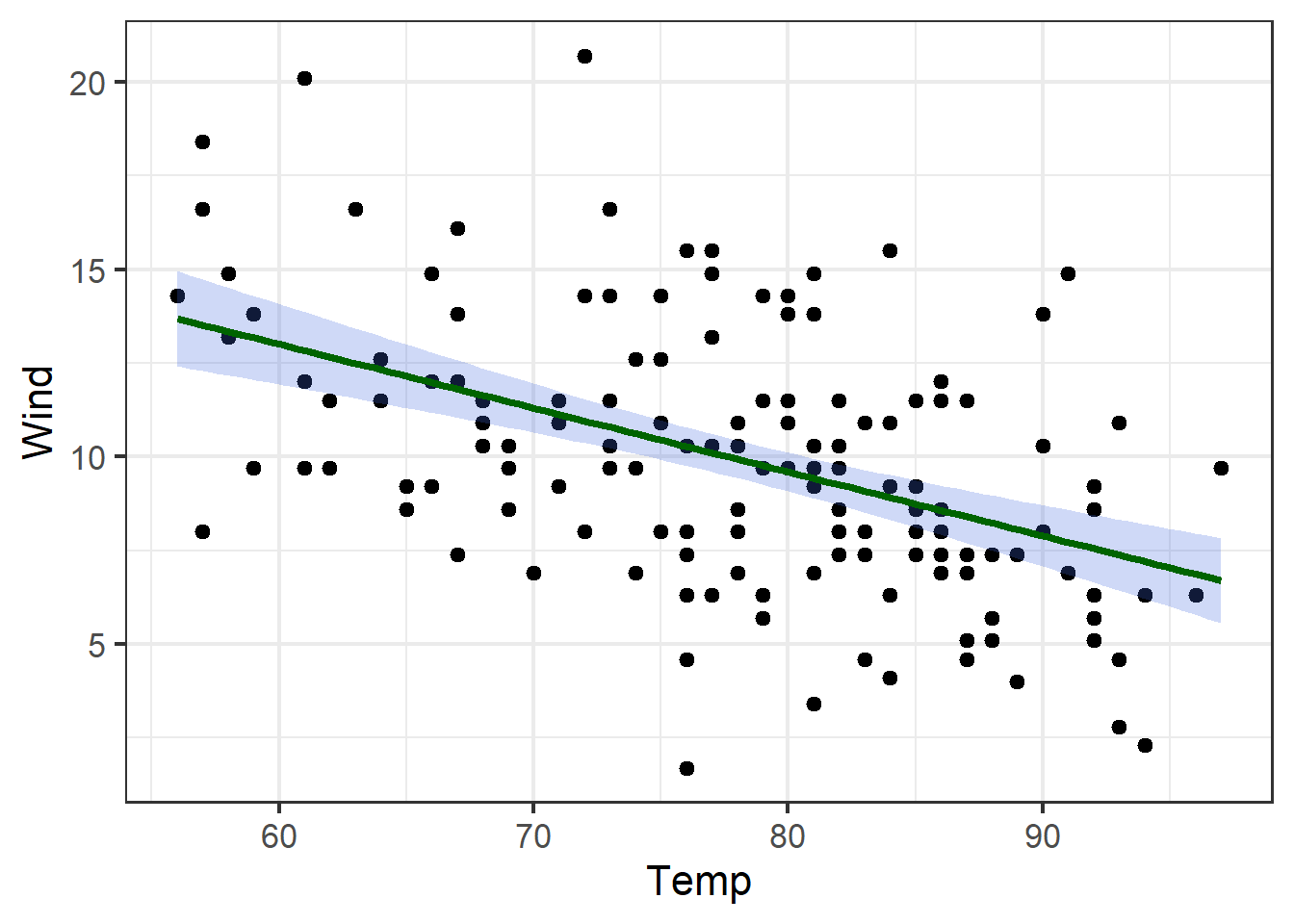
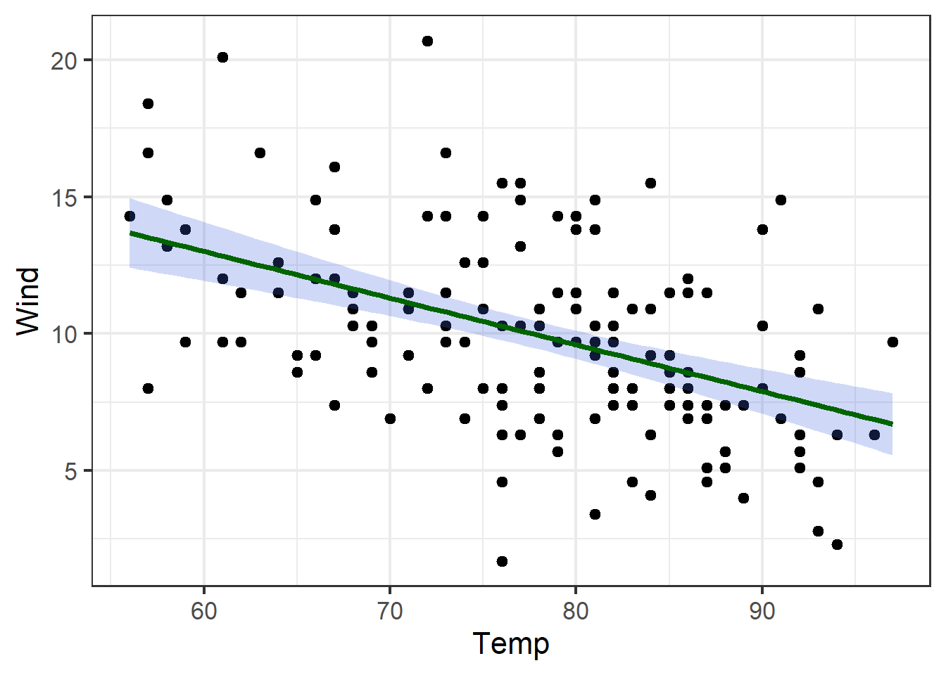
Tiếp theo câu 1, bạn hãy thêm đường trend line/regression vào đồ thị

library(ggplot2)

ggplot(data = df,
       mapping = aes(x = Temp,
                     y = Wind)) +
  
  geom_point() +
  
  geom_smooth(method = "lm",
              color = "darkgreen",
              fill = "royalblue",
              alpha = 0.25) +
  
  theme_bw(base_size = 16)

Câu 3

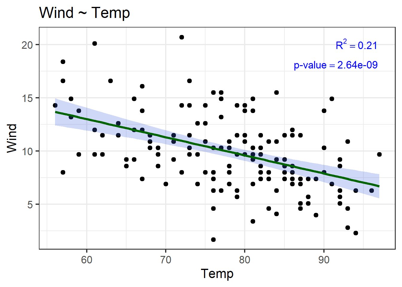
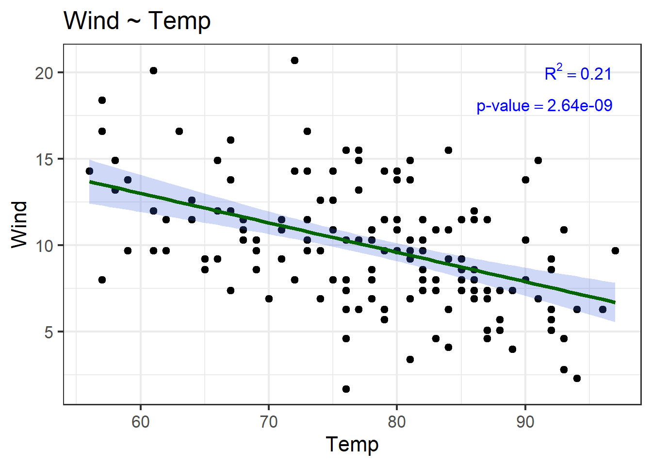
Tiếp theo câu 2, bạn hãy thêm giá trị R-squared và p-value vào đồ thị.

Đầu tiên ta cần thực hiện model hồi quy đơn biến của Wind theo Temp sau đó trích ra giá trị R-squared và p-value tương ứng.

fit <- lm(Wind ~ Temp,
          data = df)
summary(fit)

Call:
lm(formula = Wind ~ Temp, data = df)

Residuals:
   Min     1Q Median     3Q    Max 
-8.578 -2.449 -0.226  1.985  9.740 

Coefficients:
            Estimate Std. Error t value Pr(>|t|)    
(Intercept)  23.2337     2.1124   11.00  < 2e-16 ***
Temp         -0.1705     0.0269   -6.33  2.6e-09 ***
---
Signif. codes:  0 '***' 0.001 '**' 0.01 '*' 0.05 '.' 0.1 ' ' 1

Residual standard error: 3.14 on 151 degrees of freedom
Multiple R-squared:  0.21,  Adjusted R-squared:  0.205 
F-statistic: 40.1 on 1 and 151 DF,  p-value: 2.64e-09
summary(fit) -> kq

###
r_squared <- round(kq$r.squared, digits = 4)

r_squared_text <- bquote(R^2 == .(r_squared))
###

###
# tùy chỉnh tham số để thay đổi số lượng số 
# sau dấu thập phân trong p-value
options(scipen = 4)
options(digits = 3)
p_value <- kq$coefficients[2,4]

# p-value thường rất nhỏ, ggplot2 sẽ hiển thị nhiều số 0,
# ta cần chủ động chụp lại kết quả p-value trên console
p_value_ok <- capture.output(cat(p_value)) 
# p_value_ok
p_value <- p_value_ok

p_value_text <- bquote('p-value' == .(p_value))
# p_value_text 
###

Tạo đối tượng lưu text sử dụng package grid

library(ggplot2)
library(grid)

grob_r_squared_text <- grobTree(... = textGrob(label = r_squared_text, 
                          x = 0.95, 
                          y = 0.95, 
                          hjust = 1,
                          vjust = 1,
                          gp = gpar(col = "blue",
                                    fontsize = 13,
                                    fontface = "italic")))

grob_p_value_text <- grobTree(... = textGrob(label = p_value_text, 
                          x = 0.95, 
                          y = 0.85, 
                          hjust = 1,
                          vjust = 1,
                          gp = gpar(col = "blue",
                                    fontsize = 13,
                                    fontface = "italic")))

Chèn văn bản vào đồ thị sử dụng lệnh annotation_custom()
ggplot(data = df,
       mapping = aes(x = Temp,
                     y = Wind)) +
  
  geom_point() +
  
  annotation_custom(grob_r_squared_text) +
  
  annotation_custom(grob_p_value_text) +
  
  geom_smooth(method = "lm",
              color = "darkgreen",
              fill = "royalblue",
              alpha = 0.25) + 
  
  theme_bw(base_size = 16) +
  
  labs(x = "Temp",
       y = "Wind",
       title = "Wind ~ Temp")

Credit: Cảm ơn Dr. Trương Kim đã gợi ý cho mình về dạng đồ thị này.